Finding the Grid
Finding the grid turned out to be a much heftier problem than anticipated.
It is split up into two fairly orthogonal tasks: image processing to
recover corners and edges, and then setting up the grid correspondences
given the corners and edges.
Go here for some ramblings on
how edges were how to detect. Basically, because the edges are thick,
gradient-based edge detectors pick up two edges instead of one.
Instead, I developed a corner-detection algorithm specifically tweaked to
this problem. It just about never misses a corner, but occasionally an
edge might have a change in brightness on it (perhaps from a surface feature),
and that point on the edge will be labeled a corner.
The corner detector is based on the Laplacian operator. It tries different
stencils of orientations for the Laplacian's support, trying to find the
one with the best "match," which is when the Laplacian is large at one
orientation and near-zero at the "opposite orientation.
Here we can see that on the left, the Laplacian
has a very large value (oops, the figure should be 4 and -1), while on the
right, the Laplacian evaluates close to 0.
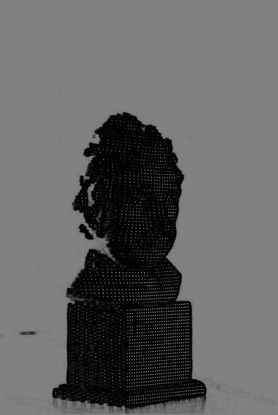
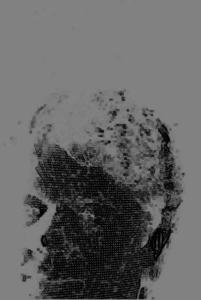
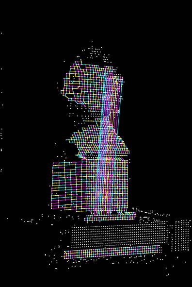
Results of corner detection in Einstein and Brett.
There is a one-to-one mapping between
points in the original grid and points projected onto the surface, as seen
by the camera.
Recovering the correspondences turned out to be much harder because the
corner extraction was not perfect. Any errors propogated to the correspondence
will not only show up as horrible artifacts in the 3-d reconstruction, but
will also wreck the correspondence algorithm, causing more bad correspondences
to domino.
The first step of the algorithm is to recover some correspondences that
are guaranteed (probabalistically) to be correct. Because we have color
information for edges that is mostly reliable, we can match multiple
edges to make the data even more reliable. A few edges may not even
map to a unique location in the original grid. We chose to search for
horizontal edges along a line because in an orthographic setup, horizontal
lines in the grid map to horizontal lines in the image. Experimentation
showed that around 12 edge-links in a row were necessary to guarantee both
uniqueness and that an error an edge labelling (or an extra or missing edge
from an extra or missing corner) didn't map to elsewhere in the original
grid.
A strip of edges got mapped incorrectly to the original grid.
Once unique horizontal strips are indentified, the correspondences propogate
outward through a breadth-first search. Edges are added if they match in
color. (The color of an edge is determined by sampling the colors near the
midpoint between the edge's two vertices.) However, because of the nearby
edges could share the same color and because there are errors in the image
processing, a more robust method is needed to guarantee that no errors
are inserted into the correspondence mapping. Instead of just looking
at one edge, we can look at multiple edges. If all agree, then with
almost always the correspondence is correct. The breadth-first search looks
for places were it can estimate the location of the next vertex (by assuming
the surface is locally planar). It then finds the nearest vertex to the
predicted location such that the edges from that vertex satisfy the correct
coloring. If the vertex is close enough to the estimated location, the
correspondence is established.
Below are several of the cases considered. On the left is the connectivity on the initial grid. On the right is the corner data. Solid arrows indicate
known correspondences. The question mark is the predicted location.
Note that for case 3, two corners are guessed, with three edge colors used
to verify. The cases are ordered in terms of robustness. The fourth case
is the least restrictive, but also the least robust. There are a few other
cases that are not shown here that are less restrictive and less robust.
They only get run if the other cases fall through and fail to extend the
correspondences.
There were a few shortcomings withthe correspondences. We were caught between keeping the algorithm conservative (so the grid never gets built incorrectly
and has to go through a costly fixing phase) and making thresholds, etc.as
liberal as possible to maximize the amount of surface recovered. Many of the
gaps in the models were from areas that were in shadow or were separated from the rest of the model by a shadow (and there was not a big enough line to
uniquely identify that component). The teapot was highly specular and
caused the thresholds for magenta to fail. Being more liberal with thresholds would certainly identify colors on more edges, but then noise in the brighter
areas would get picked up as edges.
The most important issue to address next is identifying more components from
the beginning. One possibility is to introduce more colors, such as adding
red, green, and blue. Then six color codes would be able to identify
regions uniquely with less edges. Also, instead of just looking at a
straight line and the colors of the segments along the line, we could look
at the colors of the segments branching out from along that line, although
the colors of these segments would be less accurate.
Another possiblity would be to use geographic location vertically to resolve
ambiguities in matching the horizontal lines. An energy-minimization
procedure could reduce the ambiguities to a monotonic mapping.